Why hyperdimensional computing?
DART uses hyperdimensional computing (HDC) to measure data distribution match for several reasons:
Provides a quantitative measurement of similarity
Allows for the encoding of different attribute types
Attribute Types
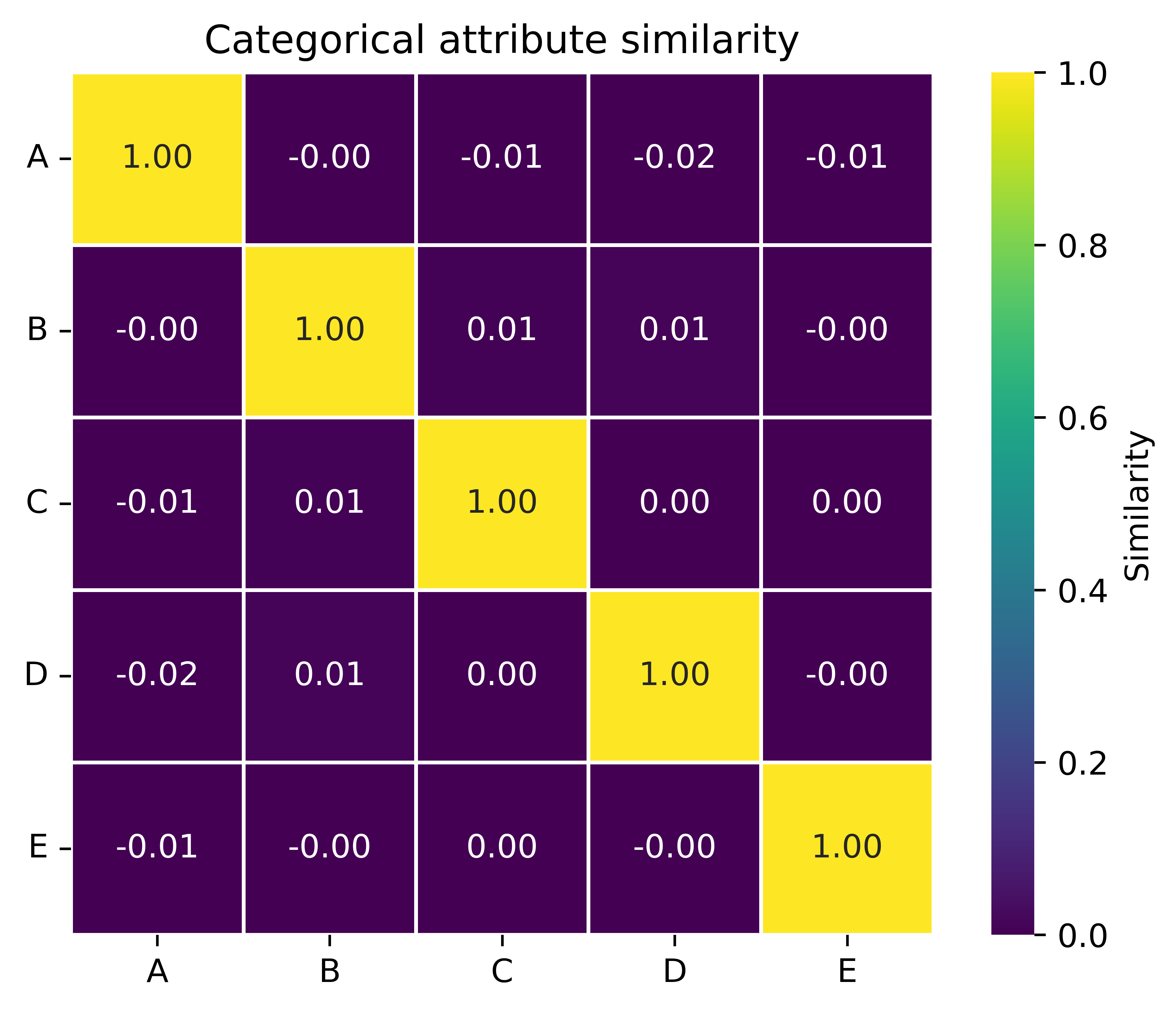
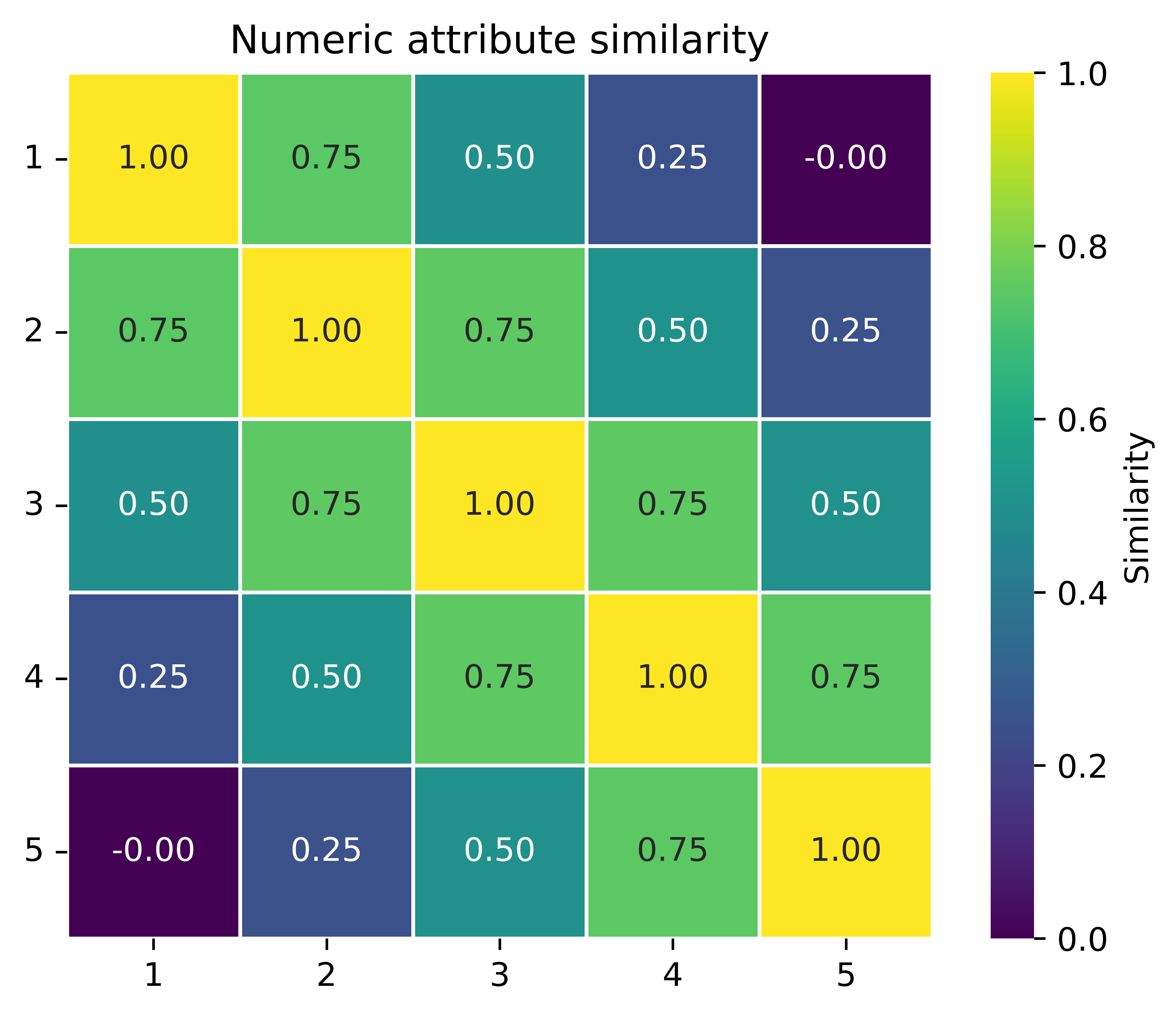
HDC allows for the creation of hypervectors with varying degrees of similarity to each other. This allows for a distinction between attributes where there is no inherent similarity between different values (e.g., categorical) and attributes where different values may have varying degrees of similarity with each other (e.g., numeric).
|
|
The similarity between any two unique values of a categorical attribute is approximately 0. The similarity between any hypervector representation and itself is always 1. |
The similarity values between any two numeric attribute values depend on their relative value. The values representing the minimum and maximum values (1 and 5, respectively) have a similarity of approximately 0. |
The importance of this property can be illustrated though the consideration of a simple toy attribute that can have the values 1, 2, 3, 4 or 5. Assume that the distribution of this attribute in “population i” needs to be compared to the two other “populations” shown in the table below.
Population |
Population values |
|---|---|
i |
2 |
ii |
5 |
iii |
3 |
The comparison can be made using a distribution similarity measurement like Jenson-Shannon distance (JSD). Such a measurement first requires converting the populations into probability distributions. Similarly, HDC requires that each population is encoded into a hypervector. Both the probability distribution and hypervector representations of the three populations are shown in the table below; the hypervectors have been shortened to fit in the table.
Population |
Probability distribution |
hypervector |
|---|---|---|
i |
[0, 1, 0, 0, 0] |
[-1, -1, -1, …, 1, 1, -1] |
ii |
[0, 0, 0, 0, 1] |
[1, 1, -1, …, 1, 1, 1] |
iii |
[0, 0, 1, 0, 0] |
[-1, 1, -1, …, 1, 1, -1] |
Finally, distributional similarity measurements are taken using Jenson-Shannon distance to measure the similarity of the probability distributions, and cosine similarity to measure the similarity of the hypervectors.
Population |
Jenson-Shannon distance |
Cosine similarity (HDC) |
|---|---|---|
ii |
0.833 |
0.016 |
iii |
0.833 |
0.254 |